Stabilizing the cart-pole system using finite-horizon LQR

There are a variety of good resources for learning LQR and various other topics in optimal control. For this post, I have referenced Russ Tedrake’s online book Underactuated Robotics and will use it in my discussion of the LQR controller and its application to stabilizing the cart-pole system within some ball of its basin of attraction. I will go through the derivation of LQR, though note that this is really well documented in Russ Tedrake’s book, and is effectively what I will follow. Afterward, I will mostly focus on solving the optimal control problem and its implementation numerically, particularly in the Julia programming language. If you are only interested in viewing the results of my implementation, feel free to scroll ahead and view the videos showing the results of the controller.

A fundamental feedback control strategy in optimal control is the linear quadratic regulator (LQR). It assumes linear dynamics of the form \(\dot{x} = Ax + Bu,\) as well as a quadratic cost function given by \(J(x,u) = h(x(T)) + \int_0^T (x^TQx + u^TRu)dt.\) It is also assumed that $Q$ is positive definite and $R$ is positive semidefinite. The Hamilton-Jacobi-Bellman (HJB) equation gives a necessary and sufficient condition for optimality for an optimal control problem. For this problem, we write the HJB as

$$0 = \underset{u}{\text{min}}\big [x^T Q x + u^T R u + \frac{\partial J^*}{\partial x}(Ax + Bu) + \frac{\partial J^*}{\partial t} \big ]. $$

With a quadratic form on $u$, there exists an optimum such that

$$\frac{\partial}{\partial u} (\text{everything inside of the min argument of the HJB}) = 2u^TR + \frac{\partial J^*}{\partial x}B = 0.$$

Solving for $u$, we arrive at

$$u^* = -\frac{1}{2}R^{-1}B^T\frac{\partial J^* }{\partial x}^T.$$

After assuming $J^* = x^T S(t) x$, we can use computations for $\frac{\partial J^* }{\partial x}$, $\frac{\partial J^* }{\partial t}$, and $u^* $ to substitute into the HJB. This will yield the continous-time differential Riccati equation:

$$ \dot{S}(t) = S(t)A + A^TS(t) -S(t) B R^{-1} B^T S(t) + Q,$$

with a terminal condition on $S(t)$ given by $S(T) = Q_f$. Again, this is all well documented at Underactuated Robotics, but let’s move to implementing these ideas on a dynamical system. The cart-pole is a common nonlinear dynamical system consisting of a cart moving along an axis, say the $x$ axis, with a pendulum attached to it. We can designate the angle of the pendulum with respect to the “down” position as $\theta$.

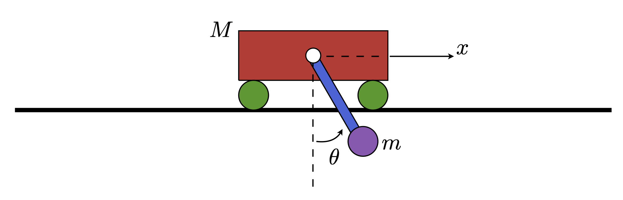
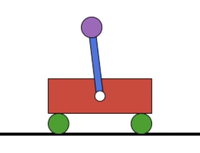
$$\text{Fig. 1. The cart-pole system.}$$

Suppose our cart-pole system is being forced in the $x$ direction, perhaps by some actuated wheels which ultimately result in forcing of the cart along the horizontal axis. We are currently working with a control strategy that works for linear(ized) time-invariant dynamical systems. This means the controller will only work within some $\epsilon$-small ball of the stable equilibrium $x^* = x_f$, $\theta^* = \pi$, $\dot{x}^* = 0$, and $\dot{\theta}^* = 0$. Firstly, assume we start within the set of LQR-controllable states. Secondly, we have some intuition of what those states are — we cannot be too far away from $\theta^* = \pi$ when employing LQR — but we do not have explicit knowledge of how far too far is. Note that one could determine this numerically for a given set of cart-pole parameters $m$, $M$, and $L$. Under no control, the the system exhibits behaviors like the one shown below.

There exist packages in MATLAB, Python, and Julia that will compute an LQR controller for you given a set of linear(ized) dynamics. I will refrain from using these tools. This is primarily because one purpose of these tutorials / posts is to solidify my understanding of these optimal control concepts. In what follows I will describe how to implement this numerically and then provide a link to my code afterward.

Our computed optimal control $u^* $ for the LQR is a function of the state $x$ as well as the time-varying funtion $S(t)$. So a question we should ask is “how do we solve for $S(t)$?” The optimal control changes as a function of $S(t)$ at each time step, so numerically we need a trajectory for $S(t)$ that corresponds to the paramters of our optimal control problem. Recall that we know a boundary condition for the continuous-time differential Riccati equation ($S(T) = Q_f$). For anyone familiar with numerically solving ODEs, finding a trajectory for $S(t)$ is simply a matter of backward simulating the continuous-time differential Riccati equation. Doing so will give us a discrete trajectory for $S(t)$, which might require that we interpolate between points not given in the solved trajectory. Or, if we are using a language like Julia, our numerical solution for $S(t)$ contains not just the solutions at discrete points in time, but an interpolating function as well. Once we have $S(t)$, we need only assume we have some mechanism allowing us full state feedback and we are clear to employ the optimal control $u^* $ as given above.

Here is a video of the resulting controller stabilizing about the point $\theta = \pi$ given the initial conditions $x(0) = 0$, $\dot{x}(0) = 0$, and $\theta(0) = \pi + \frac{\pi}{12}$, $\dot{\theta}(0) = 0$. In the spirit of my implementation in the Julia programming language, I have colorized the cart using the Julia logo colors.

The code for solving this problem can be found at Cartpole Stabilization in the cartpoleStabilization folder. Note that all of my implementations are in the Julia programming language.

Thanks for reading.