Solving the cart-pole swing-up problem with energy shaping and LQR for stabilization

In Stabilizing the cart-pole system using finite-horizon LQR, I discussed how one can implement an LQR controller to stabilize the cart-pole system when the system is initialized within the basin of attraction of the controlled system. This is satisfying in implementation, but one naturally then asks the question of how to accomplish the control problem of swinging up the pendulum when it is initialized outside of the basin of attraction. This was a neat result when I first successfully implemented it, and I still think so upon doing so a second time (in Julia).

We want to answer the question, “how can I control the system such that it possesses a certain desired amount of energy?” I again assume the parameters are all equal to 1, including the gravitational constant. Below is a video of my implementation of energy-shaping control. Continue reading for details concerning the method and implementation.

$$\text{Animation 1. A video of the final cart-pole swing-up control problem.}$$

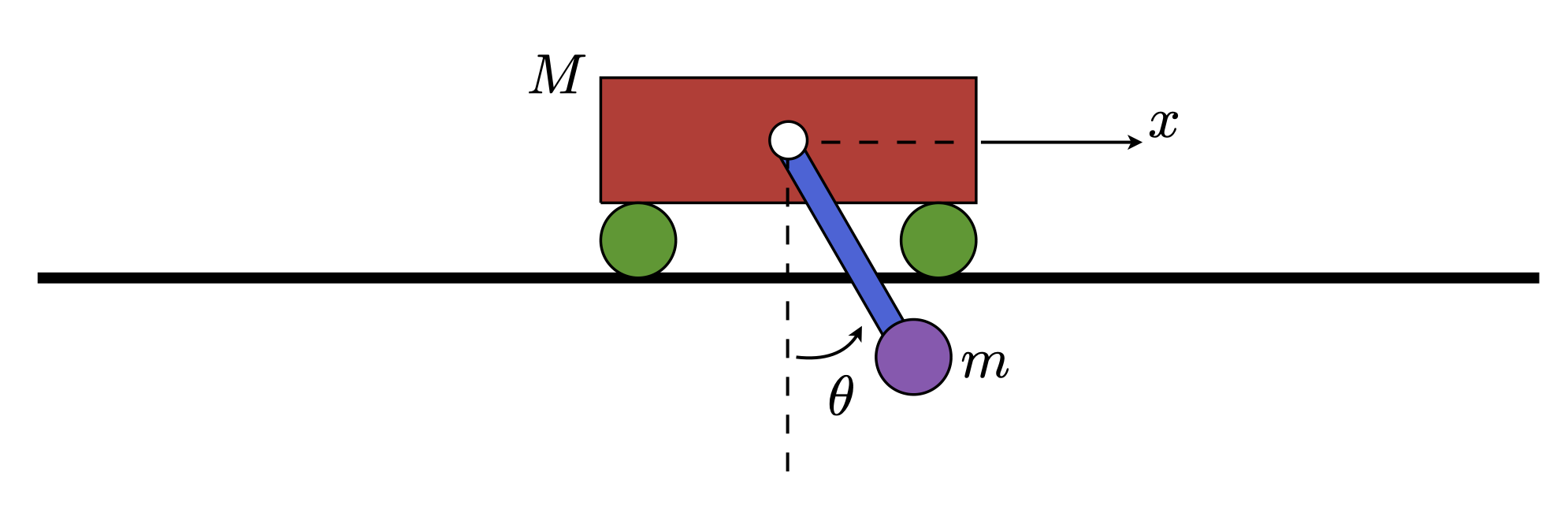
Our goal is to inject energy into the system in a controlled way such that it possesses an amount of energy corresponding to the unstable fixed point. To do this, we first need to linearize part of the dynamics so that we are working only with a subset of the nonlinear dynamics. The linearization of part of the dynamics of a system is appropriately called partial feedback linearization (PFL). There are two distinct types of PFL: collocated and non-collocated. We employ collocated PFL if we want to linearize the dynamics of actuated variables, and employ non-collocated PFL when we want to linearize the dynamics of unactuated variables. Collocated PFL yields the following equations (the same as those obtained in Underactuated Robotics when parameters are equal to 1):

$$ \ddot{\theta} = -\ddot{x}\cos\theta - \sin\theta,$$ $$ \ddot{x}(2-\cos^2\theta) - \sin\theta\cos\theta-\dot{\theta}^2\sin\theta = f_x.$$

If we apply control in the form of

$$ f_x = \ddot{x}^{des}(2-\cos^2\theta) - \sin\theta\cos\theta-\dot{\theta}^2\sin\theta, $$

then we get the partially feedback linearized equations

$$\ddot{x} = \ddot{x}^{des},$$ $$ \ddot{\theta} = -\ddot{x}^{des}\cos\theta - \sin\theta. $$

Let’s rewrite these equations such that \(u\) represents our control input.

$$\ddot{x} = u,$$ $$ \ddot{\theta} = -u\cos\theta - \sin\theta. $$

We are interested in controlling the pendulum to the unstable fixed point and to do this we need to introduce the idea of desired energy. A lone pendulum, not on a cart but rigidly affixed to the ceiling, has energy corresponding to

$$E(q,\dot{q}) = \frac{1}{2}\dot{\theta}^2 - \cos\theta. $$

This is just the kinetic energy minus the potential energy when, again, all of the parameters are equal to one. The energy at the fixed point (\(\theta = \pi\)) is

$$E(q,\dot{q}) = 1. $$

A suitable controller that injects energy into the system such that the error in the desired energy and the actual energy is zero is

$$u = k\dot{\theta}\cos\theta (E^d(q,\dot{q}) - E(q,\dot{q})).$$

However, we need to make sure the cart is regulated in some way so we superpose a PD controller for the cart and get

$$u = k_E\dot{\theta}\cos\theta (E^d(q,\dot{q}) - E(q,\dot{q})) - k_px - k_d \dot{x}.$$

I chose \(k_E = 8\), \(k_p = 0.5\), and \(k_d = 0.5\) for the controller employed in the above animation. See Underactuated Robotics for some details concerning how to ensure the energy is bounded and will go to zero. Here is a plot of the system trajectory in the phase space of the pendulum.

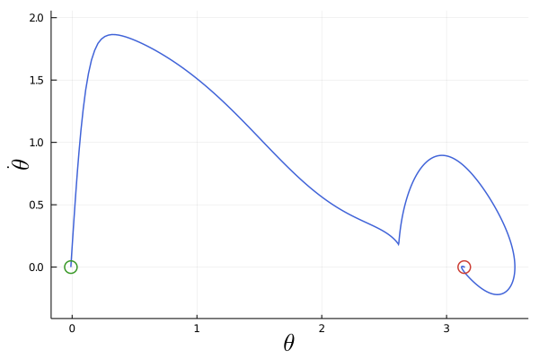
$$\text{Fig. 1. Trajectory of the pendulum in phase space under energy-shaping control.}$$

The code for solving this problem can be found at Cartpole Stabilization in the cartpoleStabilization folder. Note that all of my implementations are in the Julia programming language.

Thanks again for reading.